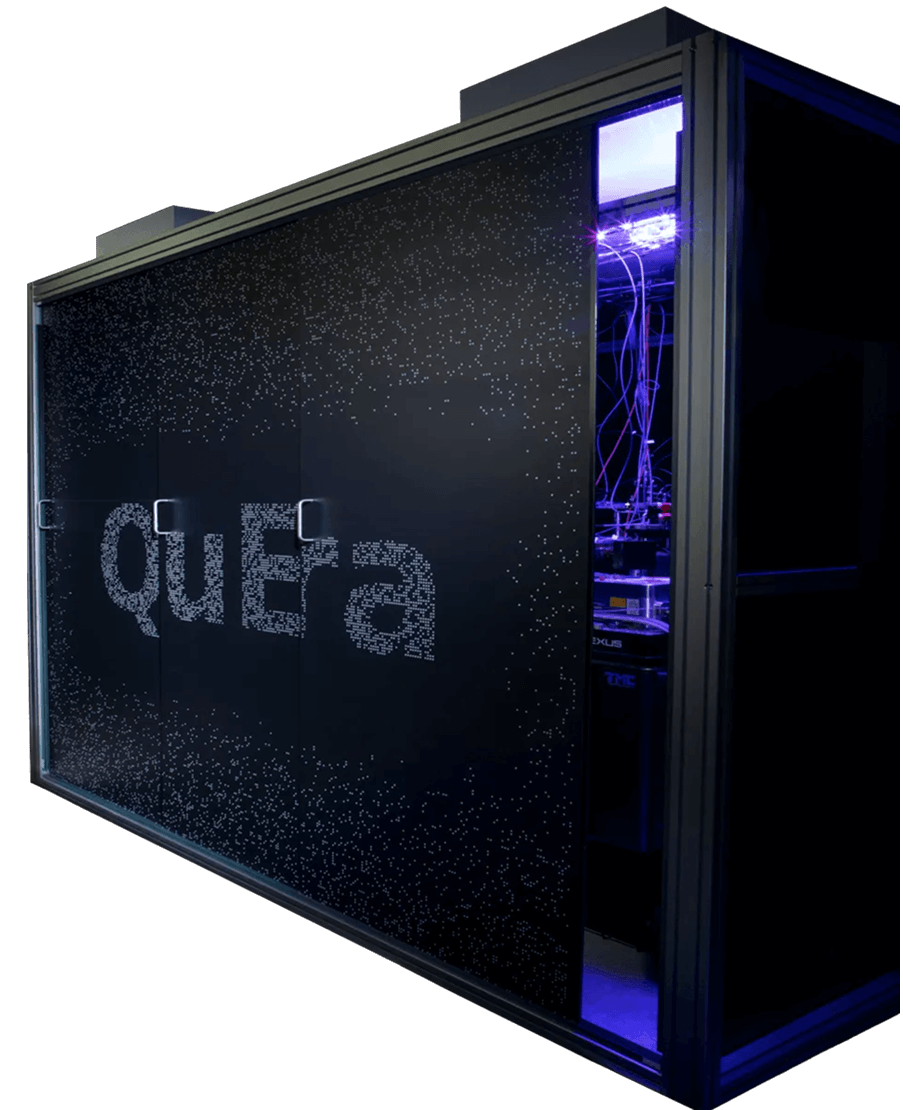
Aquila

256-Qubit Analog Neutral-Atom Quantum Computer

Dark server rack cabinet with the word 'quEra' spelled out in small white dots and a partially open door revealing cables and illuminated equipment inside.

A flexible, high-fidelity platform delivering research value today

Aquila is a field‑programmable, analog quantum processor built on a reconfigurable 256‑qubit neutral‑atom array. Launched in November 2022 as the first publicly accessible neutral‑atom quantum computer, it puts quantum to work across science and industry while establishing a foundation for future scalable systems.

White microchip icon with an orbiting electron symbol on a dark purple circular background with other faint circles.

Accessible Now

Available via Amazon Braket or via Premium Access: Secure, direct, supported environment with priority bookings.

Abstract network of glowing purple and orange circles connected by faint lines on a dark background.

Highly Flexible

Dynamic qubit layout and fine-grained analog programming enable custom-configured experiments.

Network of interconnected glowing nodes in orange and purple on a dark map-like background.

Versatile Applications

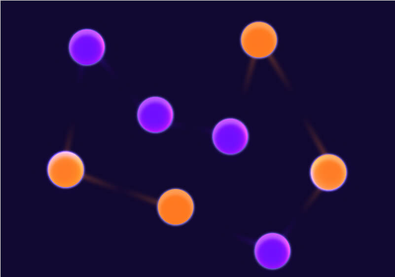
With all to all connectivity, Aquila enables unique strategies for algorithm development. Ideal for simulation, optimization, and ML workflows.

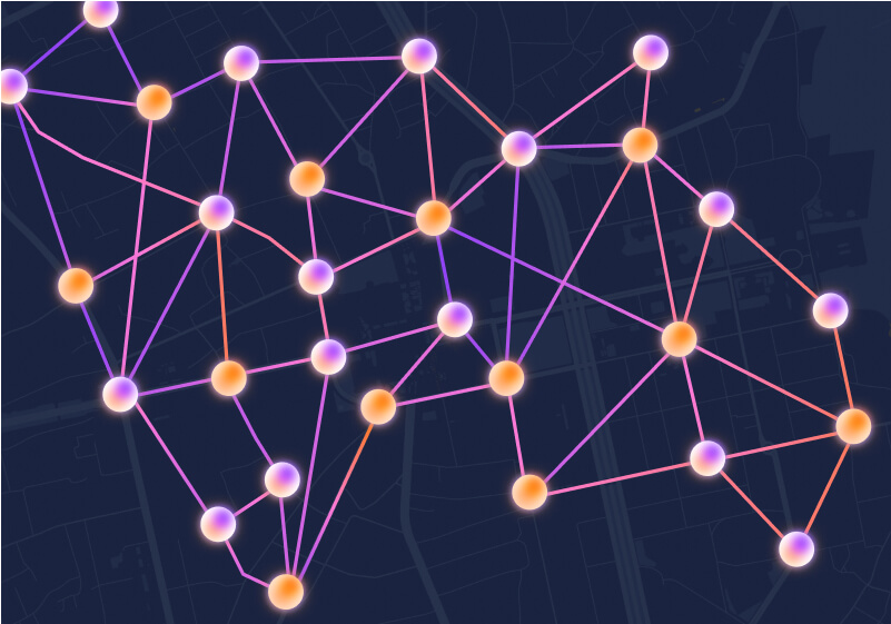
Pioneering Applications & Foundational Exploration

Aquila is more than a quantum processor—it’s a launchpad for discovery. Whether you’re advancing scientific research, solving real-world optimization, or building institutional quantum capability, Aquila delivers immediate value. Explore the examples below to see how our partners are putting quantum to work with Aquila today.

Scientific Breakthroughs

Observation of string breaking on a (2 + 1)D Rydberg quantum simulator

Read more

Real-World Usage

Robust Quantum Reservoir Learning for Molecular Property Prediction

Read more

Amazon Braket

Immediate cloud access for testing and experimentation. Aquila is available over 100 hours a week.

Premium Access

Secure access with direct support, training and guidance from QuEra scientists.

Understanding Aquila

Use our no-cost interactive training system

A comprehensive guide to neutral atom computing

Aquila on Amazon Braket

Getting started on Braket

Amazon Braket service

AWS Braket SDK

Need help?

See Examples

QuEra user forum

Amazon Braket forum

Putting Aquila Into Context

Aquila is more than a quantum processor—it’s a launchpad for discovery. Whether you’re advancing scientific research, solving real-world optimization, or building institutional quantum capability, Aquila delivers immediate value.

A large black quantum computer cabinet with 'quaEra' text made of small dots on the front panel and visible internal blue-lit cables and components.

Technical Specifications

Aquila’s analog mode operation covers a wide family of Hamiltonians within the following format:

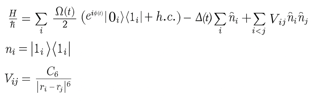
Mathematical expressions defining a Hamiltonian with sums over i and j, involving terms with Omega(t), exponential phase factors, and operators ni and Vij given by C6 divided by the sixth power of the distance between ri and rj.

General parameter ranges can be seen on the table to the right. Additional information and in-depth explanations can be found in our white paper.

Get the Aquila white paper

Parameter

Range

Processor dimensions

H: 76

W: 75

Minimal atom distance

4

Number of Qubits

256

Rabi frequency Ω

0-2.5

2π

MHz

Global rydberg detuning Δ1

-20 to 20

2π

MHz

Processor dimensions

862690

2π

MHz

^6

Abstract gradient background with smooth blend of purple, pink, and orange hues.